Extended Kalman Filter Localization
Position Estimation Kalman Filter
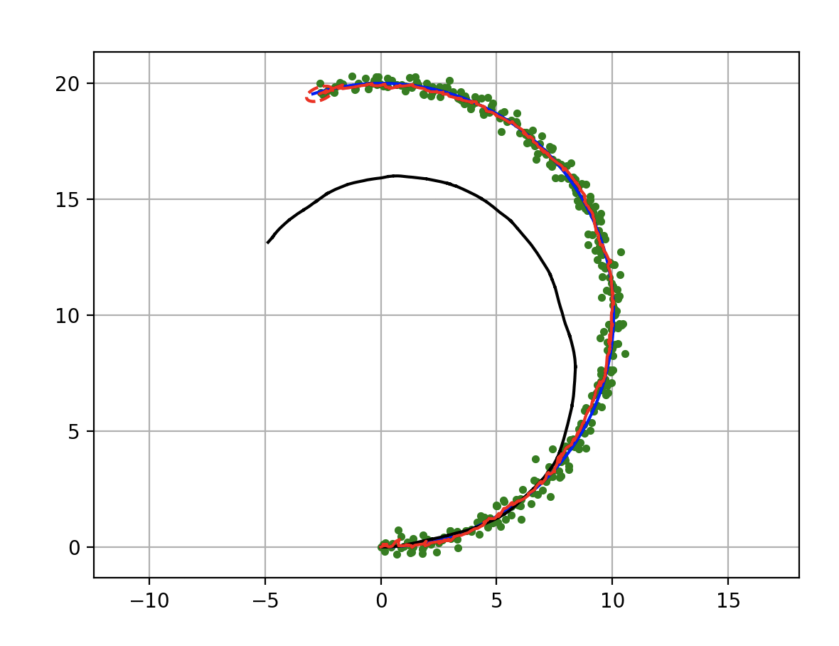

This is a sensor fusion localization with Extended Kalman Filter(EKF).
The blue line is true trajectory, the black line is dead reckoning trajectory,
the green point is positioning observation (ex. GPS), and the red line is estimated trajectory with EKF.
The red ellipse is estimated covariance ellipse with EKF.
Code: PythonRobotics/extended_kalman_filter.py at master · AtsushiSakai/PythonRobotics
Kalman Filter with Speed Scale Factor Correction
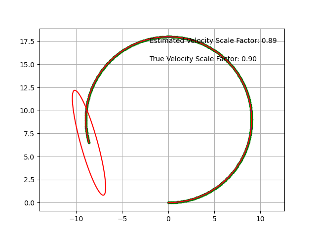
This is a Extended kalman filter (EKF) localization with velocity correction.
This is for correcting the vehicle speed measured with scale factor errors due to factors such as wheel wear.
Code: PythonRobotics/extended_kalman_ekf_with_velocity_correctionfilter.py AtsushiSakai/PythonRobotics
Filter design
Position Estimation Kalman Filter
In this simulation, the robot has a state vector includes 4 states at time \(t\).
x, y are a 2D x-y position, \(\phi\) is orientation, and v is velocity.
In the code, “xEst” means the state vector. code
And, \(P_t\) is covariace matrix of the state,
\(Q\) is covariance matrix of process noise,
\(R\) is covariance matrix of observation noise at time \(t\)
The robot has a speed sensor and a gyro sensor.
So, the input vecor can be used as each time step
Also, the robot has a GNSS sensor, it means that the robot can observe x-y position at each time.
The input and observation vector includes sensor noise.
In the code, “observation” function generates the input and observation vector with noise code
Kalman Filter with Speed Scale Factor Correction
In this simulation, the robot has a state vector includes 5 states at time \(t\).
x, y are a 2D x-y position, \(\phi\) is orientation, v is velocity, and s is a scale factor of velocity.
In the code, “xEst” means the state vector. code
The rest is the same as the Position Estimation Kalman Filter.
Motion Model
Position Estimation Kalman Filter
The robot model is
So, the motion model is
where
\(\begin{equation*} F= \begin{bmatrix} 1 & 0 & 0 & 0\\ 0 & 1 & 0 & 0\\ 0 & 0 & 1 & 0 \\ 0 & 0 & 0 & 0 \\ \end{bmatrix} \end{equation*}\)
\(\begin{equation*} B= \begin{bmatrix} cos(\phi) \Delta t & 0\\ sin(\phi) \Delta t & 0\\ 0 & \Delta t\\ 1 & 0\\ \end{bmatrix} \end{equation*}\)
\(\Delta t\) is a time interval.
This is implemented at code
The motion function is that
\(\begin{equation*} \begin{bmatrix} x' \\ y' \\ w' \\ v' \end{bmatrix} = f(\textbf{x}, \textbf{u}) = \begin{bmatrix} x + v\cos(\phi)\Delta t \\ y + v\sin(\phi)\Delta t \\ \phi + \omega \Delta t \\ v \end{bmatrix} \end{equation*}\)
Its Jacobian matrix is
\(\begin{equation*} J_f = \begin{bmatrix} \frac{\partial x'}{\partial x}& \frac{\partial x'}{\partial y} & \frac{\partial x'}{\partial \phi} & \frac{\partial x'}{\partial v}\\ \frac{\partial y'}{\partial x}& \frac{\partial y'}{\partial y} & \frac{\partial y'}{\partial \phi} & \frac{\partial y'}{\partial v}\\ \frac{\partial \phi'}{\partial x}& \frac{\partial \phi'}{\partial y} & \frac{\partial \phi'}{\partial \phi} & \frac{\partial \phi'}{\partial v}\\ \frac{\partial v'}{\partial x}& \frac{\partial v'}{\partial y} & \frac{\partial v'}{\partial \phi} & \frac{\partial v'}{\partial v} \end{bmatrix} \end{equation*}\)
\(\begin{equation*} = \begin{bmatrix} 1& 0 & -v \sin(\phi) \Delta t & \cos(\phi) \Delta t\\ 0 & 1 & v \cos(\phi) \Delta t & \sin(\phi) \Delta t\\ 0 & 0 & 1 & 0 \\ 0 & 0 & 0 & 1 \end{bmatrix} \end{equation*}\)
Kalman Filter with Speed Scale Factor Correction
The robot model is
So, the motion model is
where
\(\begin{equation*} F= \begin{bmatrix} 1 & 0 & 0 & 0 & 0\\ 0 & 1 & 0 & 0 & 0\\ 0 & 0 & 1 & 0 & 0\\ 0 & 0 & 0 & 0 & 0\\ 0 & 0 & 0 & 0 & 1\\ \end{bmatrix} \end{equation*}\)
\(\begin{equation*} B= \begin{bmatrix} cos(\phi) \Delta t s & 0\\ sin(\phi) \Delta t s & 0\\ 0 & \Delta t\\ 1 & 0\\ 0 & 0\\ \end{bmatrix} \end{equation*}\)
\(\Delta t\) is a time interval.
This is implemented at code
The motion function is that
\(\begin{equation*} \begin{bmatrix} x' \\ y' \\ w' \\ v' \end{bmatrix} = f(\textbf{x}, \textbf{u}) = \begin{bmatrix} x + v s \cos(\phi)\Delta t \\ y + v s \sin(\phi)\Delta t \\ \phi + \omega \Delta t \\ v \end{bmatrix} \end{equation*}\)
Its Jacobian matrix is
\(\begin{equation*} J_f = \begin{bmatrix} \frac{\partial x'}{\partial x}& \frac{\partial x'}{\partial y} & \frac{\partial x'}{\partial \phi} & \frac{\partial x'}{\partial v} & \frac{\partial x'}{\partial s}\\ \frac{\partial y'}{\partial x}& \frac{\partial y'}{\partial y} & \frac{\partial y'}{\partial \phi} & \frac{\partial y'}{\partial v} & \frac{\partial y'}{\partial s}\\ \frac{\partial \phi'}{\partial x}& \frac{\partial \phi'}{\partial y} & \frac{\partial \phi'}{\partial \phi} & \frac{\partial \phi'}{\partial v} & \frac{\partial \phi'}{\partial s}\\ \frac{\partial v'}{\partial x}& \frac{\partial v'}{\partial y} & \frac{\partial v'}{\partial \phi} & \frac{\partial v'}{\partial v} & \frac{\partial v'}{\partial s} \\ \frac{\partial s'}{\partial x}& \frac{\partial s'}{\partial y} & \frac{\partial s'}{\partial \phi} & \frac{\partial s'}{\partial v} & \frac{\partial s'}{\partial s} \end{bmatrix} \end{equation*}\)
\(\begin{equation*} = \begin{bmatrix} 1& 0 & -v s \sin(\phi) \Delta t & s \cos(\phi) \Delta t & \cos(\phi) v \Delta t\\ 0 & 1 & v s \cos(\phi) \Delta t & s \sin(\phi) \Delta t & v \sin(\phi) \Delta t\\ 0 & 0 & 1 & 0 & 0 \\ 0 & 0 & 0 & 1 & 0 \end{bmatrix} \end{equation*}\)
Observation Model
Position Estimation Kalman Filter
The robot can get x-y position infomation from GPS.
So GPS Observation model is
where
\(\begin{equation*} H = \begin{bmatrix} 1 & 0 & 0 & 0 \\ 0 & 1 & 0 & 0 \\ \end{bmatrix} \end{equation*}\)
The observation function states that
\(\begin{equation*} \begin{bmatrix} x' \\ y' \end{bmatrix} = g(\textbf{x}) = \begin{bmatrix} x \\ y \end{bmatrix} \end{equation*}\)
Its Jacobian matrix is
\(\begin{equation*} J_g = \begin{bmatrix} \frac{\partial x'}{\partial x} & \frac{\partial x'}{\partial y} & \frac{\partial x'}{\partial \phi} & \frac{\partial x'}{\partial v}\\ \frac{\partial y'}{\partial x}& \frac{\partial y'}{\partial y} & \frac{\partial y'}{\partial \phi} & \frac{\partial y'}{ \partial v}\\ \end{bmatrix} \end{equation*}\)
\(\begin{equation*} = \begin{bmatrix} 1& 0 & 0 & 0\\ 0 & 1 & 0 & 0\\ \end{bmatrix} \end{equation*}\)
Kalman Filter with Speed Scale Factor Correction
The robot can get x-y position infomation from GPS.
So GPS Observation model is
where
\(\begin{equation*} H = \begin{bmatrix} 1 & 0 & 0 & 0 & 0 \\ 0 & 1 & 0 & 0 & 0 \\ \end{bmatrix} \end{equation*}\)
The observation function states that
\(\begin{equation*} \begin{bmatrix} x' \\ y' \end{bmatrix} = g(\textbf{x}) = \begin{bmatrix} x \\ y \end{bmatrix} \end{equation*}\)
Its Jacobian matrix is
\(\begin{equation*} J_g = \begin{bmatrix} \frac{\partial x'}{\partial x} & \frac{\partial x'}{\partial y} & \frac{\partial x'}{\partial \phi} & \frac{\partial x'}{\partial v} & \frac{\partial x'}{\partial s}\\ \frac{\partial y'}{\partial x}& \frac{\partial y'}{\partial y} & \frac{\partial y'}{\partial \phi} & \frac{\partial y'}{ \partial v} & \frac{\partial y'}{ \partial s}\\ \end{bmatrix} \end{equation*}\)
\(\begin{equation*} = \begin{bmatrix} 1& 0 & 0 & 0 & 0\\ 0 & 1 & 0 & 0 & 0\\ \end{bmatrix} \end{equation*}\)
Extended Kalman Filter
Localization process using Extended Kalman Filter:EKF is
=== Predict ===
\(x_{Pred} = Fx_t+Bu_t\)
\(P_{Pred} = J_f P_t J_f^T + Q\)
=== Update ===
\(z_{Pred} = Hx_{Pred}\)
\(y = z - z_{Pred}\)
\(S = J_g P_{Pred}.J_g^T + R\)
\(K = P_{Pred}.J_g^T S^{-1}\)
\(x_{t+1} = x_{Pred} + Ky\)
\(P_{t+1} = ( I - K J_g) P_{Pred}\)