Inverted Pendulum Control

An inverted pendulum on a cart consists of a mass \(m\) at the top of a pole of length \(l\) pivoted on a horizontally moving base as shown in the adjacent.

The objective of the control system is to balance the inverted pendulum by applying a force to the cart that the pendulum is attached to.

Modeling

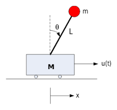
• \(M\): mass of the cart

• \(m\): mass of the load on the top of the rod

• \(l\): length of the rod

• \(u\): force applied to the cart

• \(x\): cart position coordinate

• \(\theta\): pendulum angle from vertical

Using Lagrange’s equations:

\[\begin{split}& (M + m)\ddot{x} - ml\ddot{\theta}cos{\theta} + ml\dot{\theta^2}\sin{\theta} = u \\ & l\ddot{\theta} - g\sin{\theta} = \ddot{x}\cos{\theta}\end{split}\]

See this link for more details.

So

\[\begin{split}& \ddot{x} = \frac{m(gcos{\theta} - \dot{\theta}^2l)sin{\theta} + u}{M + m - mcos^2{\theta}} \\ & \ddot{\theta} = \frac{g(M + m)sin{\theta} - \dot{\theta}^2lmsin{\theta}cos{\theta} + ucos{\theta}}{l(M + m - mcos^2{\theta})}\end{split}\]

Linearized model when \(\theta\) small, \(cos{\theta} \approx 1\), \(sin{\theta} \approx \theta\), \(\dot{\theta}^2 \approx 0\).

\[\begin{split}& \ddot{x} = \frac{gm}{M}\theta + \frac{1}{M}u\\ & \ddot{\theta} = \frac{g(M + m)}{Ml}\theta + \frac{1}{Ml}u\end{split}\]

State space:

\[\begin{split}& \dot{x} = Ax + Bu \\ & y = Cx + Du\end{split}\]

where

\[\begin{split}& x = [x, \dot{x}, \theta,\dot{\theta}]\\ & A = \begin{bmatrix} 0 & 1 & 0 & 0\\0 & 0 & \frac{gm}{M} & 0\\0 & 0 & 0 & 1\\0 & 0 & \frac{g(M + m)}{Ml} & 0 \end{bmatrix}\\ & B = \begin{bmatrix} 0 \\ \frac{1}{M} \\ 0 \\ \frac{1}{Ml} \end{bmatrix}\end{split}\]

If control only theta

\[\begin{split}& C = \begin{bmatrix} 0 & 0 & 1 & 0 \end{bmatrix}\\ & D = [0]\end{split}\]

If control x and theta

\[\begin{split}& C = \begin{bmatrix} 1 & 0 & 0 & 0\\0 & 0 & 1 & 0 \end{bmatrix}\\ & D = \begin{bmatrix} 0 \\ 0 \end{bmatrix}\end{split}\]

LQR control

The LQR controller minimize this cost function defined as:

\[J = x^T Q x + u^T R u\]

the feedback control law that minimizes the value of the cost is:

\[u = -K x\]

where:

\[K = (B^T P B + R)^{-1} B^T P A\]

and \(P\) is the unique positive definite solution to the discrete time algebraic Riccati equation (DARE):

\[P = A^T P A - A^T P B ( R + B^T P B )^{-1} B^T P A + Q\]

MPC control

The MPC controller minimize this cost function defined as:

\[J = x^T Q x + u^T R u\]

subject to:

• Linearized Inverted Pendulum model

• Initial state