Graph based SLAM
This is a graph based SLAM example.
The blue line is ground truth.
The black line is dead reckoning.
The red line is the estimated trajectory with Graph based SLAM.
The black stars are landmarks for graph edge generation.

Graph SLAM
import copy
import math
import itertools
import numpy as np
import matplotlib.pyplot as plt
from graph_based_slam import calc_rotational_matrix, calc_jacobian, cal_observation_sigma, \
                             calc_input, observation, motion_model, Edge, pi_2_pi

%matplotlib inline
np.set_printoptions(precision=3, suppress=True)
np.random.seed(0)
Introduction
In contrast to the probabilistic approaches for solving SLAM, such as EKF, UKF, particle filters, and so on, the graph technique formulates the SLAM as an optimization problem. It is mostly used to solve the full SLAM problem in an offline fashion, i.e. optimize all the poses of the robot after the path has been traversed. However, some variants are available that uses graph-based approaches to perform online estimation or to solve for a subset of the poses.
GraphSLAM uses the motion information as well as the observations of the environment to create least square problem that can be solved using standard optimization techniques.
Minimal Example
The following example illustrates the main idea behind graphSLAM. A simple case of a 1D robot is considered that can only move in 1 direction. The robot is commanded to move forward with a control input \(u_t=1\), however, the motion is not perfect and the measured odometry will deviate from the true path. At each time step the robot can observe its environment, for this simple case as well, there is only a single landmark at coordinates \(x=3\). The measured observations are the range between the robot and landmark. These measurements are also subjected to noise. No bearing information is required since this is a 1D problem.
To solve this, graphSLAM creates what is called as the system information matrix \(\Omega\) also referred to as \(H\) and the information vector \(\xi\) also known as \(b\). The entries are created based on the information of the motion and the observation.
R = 0.2
Q = 0.2
N = 3
graphics_radius = 0.1

odom = np.empty((N,1))
obs = np.empty((N,1))
x_true = np.empty((N,1))

landmark = 3
# Simulated readings of odometry and observations
x_true[0], odom[0], obs[0] = 0.0, 0.0, 2.9
x_true[1], odom[1], obs[1] = 1.0, 1.5, 2.0
x_true[2], odom[2], obs[2] = 2.0, 2.4, 1.0

hxDR = copy.deepcopy(odom)
# Visualization
plt.plot(landmark,0, '*k', markersize=30)
for i in range(N):
    plt.plot(odom[i], 0, '.', markersize=50, alpha=0.8, color='steelblue')
    plt.plot([odom[i], odom[i] + graphics_radius],
             [0,0], 'r')
    plt.text(odom[i], 0.02, "X_{}".format(i), fontsize=12)
    plt.plot(obs[i]+odom[i],0,'.', markersize=25, color='brown')
    plt.plot(x_true[i],0,'.g', markersize=20)
plt.grid()
plt.show()


# Defined as a function to facilitate iteration
def get_H_b(odom, obs):
    """
    Create the information matrix and information vector. This implementation is
    based on the concept of virtual measurement i.e. the observations of the
    landmarks are converted into constraints (edges) between the nodes that
    have observed this landmark.
    """
    measure_constraints = {}
    omegas = {}
    zids = list(itertools.combinations(range(N),2))
    H = np.zeros((N,N))
    b = np.zeros((N,1))
    for (t1, t2) in zids:
        x1 = odom[t1]
        x2 = odom[t2]
        z1 = obs[t1]
        z2 = obs[t2]

        # Adding virtual measurement constraint
        measure_constraints[(t1,t2)] = (x2-x1-z1+z2)
        omegas[(t1,t2)] = (1 / (2*Q))

        # populate system's information matrix and vector
        H[t1,t1] += omegas[(t1,t2)]
        H[t2,t2] += omegas[(t1,t2)]
        H[t2,t1] -= omegas[(t1,t2)]
        H[t1,t2] -= omegas[(t1,t2)]

        b[t1] += omegas[(t1,t2)] * measure_constraints[(t1,t2)]
        b[t2] -= omegas[(t1,t2)] * measure_constraints[(t1,t2)]

    return H, b


H, b = get_H_b(odom, obs)
print("The determinant of H: ", np.linalg.det(H))
H[0,0] += 1 # np.inf ?
print("The determinant of H after anchoring constraint: ", np.linalg.det(H))

for i in range(5):
    H, b = get_H_b(odom, obs)
    H[(0,0)] += 1

    # Recover the posterior over the path
    dx = np.linalg.inv(H) @ b
    odom += dx
    # repeat till convergence
print("Running graphSLAM ...")
print("Odometry values after optimzation: \n", odom)

plt.figure()
plt.plot(x_true, np.zeros(x_true.shape), '.', markersize=20, label='Ground truth')
plt.plot(odom, np.zeros(x_true.shape), '.', markersize=20, label='Estimation')
plt.plot(hxDR, np.zeros(x_true.shape), '.', markersize=20, label='Odom')
plt.legend()
plt.grid()
plt.show()
The determinant of H:  0.0
The determinant of H after anchoring constraint:  18.750000000000007
Running graphSLAM ...
Odometry values after optimzation:
 [[-0. ]
 [ 0.9]
 [ 1.9]]
In particular, the tasks are split into 2 parts, graph construction, and graph optimization. ### Graph Construction
Firstly the nodes are defined \(\boldsymbol{x} = \boldsymbol{x}_{1:n}\) such that each node is the pose of the robot at time \(t_i\) Secondly, the edges i.e. the constraints, are constructed according to the following conditions:
robot moves from \(\boldsymbol{x}_i\) to \(\boldsymbol{x}_j\). This edge corresponds to the odometry measurement. Relative motion constraints (Not included in the previous minimal example).
Measurement constraints, this can be done in two ways:
The information matrix is set in such a way that it includes the landmarks in the map as well. Then the constraints can be entered in a straightforward fashion between a node \(\boldsymbol{x}_i\) and some landmark \(m_k\)
Through creating a virtual measurement among all the node that have observed the same landmark. More concretely, robot observes the same landmark from \(\boldsymbol{x}_i\) and \(\boldsymbol{x}_j\). Relative measurement constraint. The “virtual measurement” \(\boldsymbol{z}_{ij}\), which is the estimated pose of \(\boldsymbol{x}_j\) as seen from the node \(\boldsymbol{x}_i\). The virtual measurement can then be entered in the information matrix and vector in a similar fashion to the motion constraints.
An edge is fully characterized by the values of the error (entry to information vector) and the local information matrix (entry to the system’s information vector). The larger the local information matrix (lower \(Q\) or \(R\)) the values that this edge will contribute with.
Important Notes:
The addition to the information matrix and vector are added to the earlier values.
In the case of 2D robot, the constraints will be non-linear, therefore, a Jacobian of the error w.r.t the states is needed when updated \(H\) and \(b\).
The anchoring constraint is needed in order to avoid having a singular information matri.
Graph Optimization
The result from this formulation yields an overdetermined system of equations. The goal after constructing the graph is to find: \(x^*=\underset{x}{\mathrm{argmin}}~\underset{ij}\Sigma~f(e_{ij})\), where \(f\) is some error function that depends on the edges between to related nodes \(i\) and \(j\). The derivation in the references arrive at the solution for \(x^* = H^{-1}b\)
Planar Example:
Now we will go through an example with a more realistic case of a 2D robot with 3DoF, namely, \([x, y, \theta]^T\)
#  Simulation parameter
Qsim = np.diag([0.01, np.deg2rad(0.010)])**2 # error added to range and bearing
Rsim = np.diag([0.1, np.deg2rad(1.0)])**2 # error added to [v, w]

DT = 2.0  # time tick [s]
SIM_TIME = 100.0  # simulation time [s]
MAX_RANGE = 30.0  # maximum observation range
STATE_SIZE = 3  # State size [x,y,yaw]

# TODO: Why not use Qsim ?
# Covariance parameter of Graph Based SLAM
C_SIGMA1 = 0.1
C_SIGMA2 = 0.1
C_SIGMA3 = np.deg2rad(1.0)

MAX_ITR = 20  # Maximum iteration during optimization
timesteps = 1

# consider only 2 landmarks for simplicity
# RFID positions [x, y, yaw]
RFID = np.array([[10.0, -2.0, 0.0],
#                  [15.0, 10.0, 0.0],
#                  [3.0, 15.0, 0.0],
#                  [-5.0, 20.0, 0.0],
#                  [-5.0, 5.0, 0.0]
                 ])

# State Vector [x y yaw v]'
xTrue = np.zeros((STATE_SIZE, 1))
xDR = np.zeros((STATE_SIZE, 1))  # Dead reckoning
xTrue[2] = np.deg2rad(45)
xDR[2] = np.deg2rad(45)
# history initial values
hxTrue = xTrue
hxDR = xTrue
_, z, _, _ = observation(xTrue, xDR, np.array([[0,0]]).T, RFID)
hz = [z]

for i in range(timesteps):
    u = calc_input()
    xTrue, z, xDR, ud = observation(xTrue, xDR, u, RFID)
    hxDR = np.hstack((hxDR, xDR))
    hxTrue = np.hstack((hxTrue, xTrue))
    hz.append(z)

# visualize
graphics_radius = 0.3
plt.plot(RFID[:, 0], RFID[:, 1], "*k", markersize=20)
plt.plot(hxDR[0, :], hxDR[1, :], '.', markersize=50, alpha=0.8, label='Odom')
plt.plot(hxTrue[0, :], hxTrue[1, :], '.', markersize=20, alpha=0.6, label='X_true')

for i in range(hxDR.shape[1]):
    x = hxDR[0, i]
    y = hxDR[1, i]
    yaw = hxDR[2, i]
    plt.plot([x, x + graphics_radius * np.cos(yaw)],
             [y, y + graphics_radius * np.sin(yaw)], 'r')
    d = hz[i][:, 0]
    angle = hz[i][:, 1]
    plt.plot([x + d * np.cos(angle + yaw)], [y + d * np.sin(angle + yaw)], '.',
             markersize=20, alpha=0.7)
    plt.legend()
plt.grid()
plt.show()
# Copy the data to have a consistent naming with the .py file
zlist = copy.deepcopy(hz)
x_opt = copy.deepcopy(hxDR)
xlist = copy.deepcopy(hxDR)
number_of_nodes = x_opt.shape[1]
n = number_of_nodes * STATE_SIZE
After the data has been saved, the graph will be constructed by looking at each pair for nodes. The virtual measurement is only created if two nodes have observed the same landmark at different points in time. The next cells are a walk through for a single iteration of graph construction -> optimization -> estimate update.
# get all the possible combination of the different node
zids = list(itertools.combinations(range(len(zlist)), 2))
print("Node combinations: \n", zids)

for i in range(xlist.shape[1]):
    print("Node {} observed landmark with ID {}".format(i, zlist[i][0, 3]))
Node combinations:
 [(0, 1)]
Node 0 observed landmark with ID 0.0
Node 1 observed landmark with ID 0.0
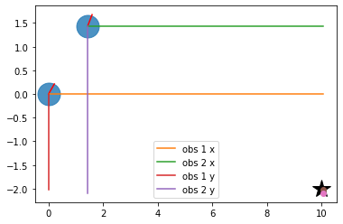
In the following code snippet the error based on the virtual measurement between node 0 and 1 will be created. The equations for the error is as follows: \(e_{ij}^x = x_j + d_j cos(\psi_j +\theta_j) - x_i - d_i cos(\psi_i + \theta_i)\)
\(e_{ij}^y = y_j + d_j sin(\psi_j + \theta_j) - y_i - d_i sin(\psi_i + \theta_i)\)
\(e_{ij}^x = \psi_j + \theta_j - \psi_i - \theta_i\)
Where \([x_i, y_i, \psi_i]\) is the pose for node \(i\) and similarly for node \(j\), \(d\) is the measured distance at nodes \(i\) and \(j\), and \(\theta\) is the measured bearing to the landmark. The difference is visualized with the figure in the next cell.
In case of perfect motion and perfect measurement the error shall be zero since \(x_j + d_j cos(\psi_j + \theta_j)\) should equal \(x_i + d_i cos(\psi_i + \theta_i)\)
# Initialize edges list
edges = []

# Go through all the different combinations
for (t1, t2) in zids:
    x1, y1, yaw1 = xlist[0, t1], xlist[1, t1], xlist[2, t1]
    x2, y2, yaw2 = xlist[0, t2], xlist[1, t2], xlist[2, t2]

    # All nodes have valid observation with ID=0, therefore, no data association condition
    iz1 = 0
    iz2 = 0

    d1 = zlist[t1][iz1, 0]
    angle1, phi1 = zlist[t1][iz1, 1], zlist[t1][iz1, 2]
    d2 = zlist[t2][iz2, 0]
    angle2, phi2 = zlist[t2][iz2, 1], zlist[t2][iz2, 2]

    # find angle between observation and horizontal
    tangle1 = pi_2_pi(yaw1 + angle1)
    tangle2 = pi_2_pi(yaw2 + angle2)

    # project the observations
    tmp1 = d1 * math.cos(tangle1)
    tmp2 = d2 * math.cos(tangle2)
    tmp3 = d1 * math.sin(tangle1)
    tmp4 = d2 * math.sin(tangle2)

    edge = Edge()
    print(y1,y2, tmp3, tmp4)
    # calculate the error of the virtual measurement
    # node 1 as seen from node 2 throught the observations 1,2
    edge.e[0, 0] = x2 - x1 - tmp1 + tmp2
    edge.e[1, 0] = y2 - y1 - tmp3 + tmp4
    edge.e[2, 0] = pi_2_pi(yaw2 - yaw1 - tangle1 + tangle2)

    edge.d1, edge.d2 = d1, d2
    edge.yaw1, edge.yaw2 = yaw1, yaw2
    edge.angle1, edge.angle2 = angle1, angle2
    edge.id1, edge.id2 = t1, t2

    edges.append(edge)

    print("For nodes",(t1,t2))
    print("Added edge with errors: \n", edge.e)

    # Visualize measurement projections
    plt.plot(RFID[0, 0], RFID[0, 1], "*k", markersize=20)
    plt.plot([x1,x2],[y1,y2], '.', markersize=50, alpha=0.8)
    plt.plot([x1, x1 + graphics_radius * np.cos(yaw1)],
             [y1, y1 + graphics_radius * np.sin(yaw1)], 'r')
    plt.plot([x2, x2 + graphics_radius * np.cos(yaw2)],
             [y2, y2 + graphics_radius * np.sin(yaw2)], 'r')

    plt.plot([x1,x1+tmp1], [y1,y1], label="obs 1 x")
    plt.plot([x2,x2+tmp2], [y2,y2], label="obs 2 x")
    plt.plot([x1,x1], [y1,y1+tmp3], label="obs 1 y")
    plt.plot([x2,x2], [y2,y2+tmp4], label="obs 2 y")
    plt.plot(x1+tmp1, y1+tmp3, 'o')
    plt.plot(x2+tmp2, y2+tmp4, 'o')
plt.legend()
plt.grid()
plt.show()
0.0 1.427649841628278 -2.0126109674819155 -3.524048014922737
For nodes (0, 1)
Added edge with errors:
 [[-0.02 ]
 [-0.084]
 [ 0.   ]]
Since the constraints equations derived before are non-linear, linearization is needed before we can insert them into the information matrix and information vector. Two jacobians
\(A = \frac{\partial e_{ij}}{\partial \boldsymbol{x}_i}\) as \(\boldsymbol{x}_i\) holds the three variabls x, y, and theta. Similarly, \(B = \frac{\partial e_{ij}}{\partial \boldsymbol{x}_j}\)
# Initialize the system information matrix and information vector
H = np.zeros((n, n))
b = np.zeros((n, 1))
x_opt = copy.deepcopy(hxDR)
for edge in edges:
id1 = edge.id1 * STATE_SIZE
id2 = edge.id2 * STATE_SIZE
t1 = edge.yaw1 + edge.angle1
A = np.array([[-1.0, 0, edge.d1 * math.sin(t1)],
[0, -1.0, -edge.d1 * math.cos(t1)],
[0, 0, -1.0]])
t2 = edge.yaw2 + edge.angle2
B = np.array([[1.0, 0, -edge.d2 * math.sin(t2)],
[0, 1.0, edge.d2 * math.cos(t2)],
[0, 0, 1.0]])
# TODO: use Qsim instead of sigma
sigma = np.diag([C_SIGMA1, C_SIGMA2, C_SIGMA3])
Rt1 = calc_rotational_matrix(tangle1)
Rt2 = calc_rotational_matrix(tangle2)
edge.omega = np.linalg.inv(Rt1 @ sigma @ Rt1.T + Rt2 @ sigma @ Rt2.T)
# Fill in entries in H and b
H[id1:id1 + STATE_SIZE, id1:id1 + STATE_SIZE] += A.T @ edge.omega @ A
H[id1:id1 + STATE_SIZE, id2:id2 + STATE_SIZE] += A.T @ edge.omega @ B
H[id2:id2 + STATE_SIZE, id1:id1 + STATE_SIZE] += B.T @ edge.omega @ A
H[id2:id2 + STATE_SIZE, id2:id2 + STATE_SIZE] += B.T @ edge.omega @ B
b[id1:id1 + STATE_SIZE] += (A.T @ edge.omega @ edge.e)
b[id2:id2 + STATE_SIZE] += (B.T @ edge.omega @ edge.e)
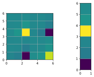
print("The determinant of H: ", np.linalg.det(H))
plt.figure()
plt.subplot(1,2,1)
plt.imshow(H, extent=[0, n, 0, n])
plt.subplot(1,2,2)
plt.imshow(b, extent=[0, 1, 0, n])
plt.show()
# Fix the origin, multiply by large number gives same results but better visualization
H[0:STATE_SIZE, 0:STATE_SIZE] += np.identity(STATE_SIZE)
print("The determinant of H after origin constraint: ", np.linalg.det(H))
plt.figure()
plt.subplot(1,2,1)
plt.imshow(H, extent=[0, n, 0, n])
plt.subplot(1,2,2)
plt.imshow(b, extent=[0, 1, 0, n])
plt.show()
The determinant of H:  0.0
The determinant of H after origin constraint:  716.1972439134893

# Find the solution (first iteration)
dx = - np.linalg.inv(H) @ b
for i in range(number_of_nodes):
    x_opt[0:3, i] += dx[i * 3:i * 3 + 3, 0]
print("dx: \n",dx)
print("ground truth: \n ",hxTrue)
print("Odom: \n", hxDR)
print("SLAM: \n", x_opt)

# performance will improve with more iterations, nodes and landmarks.
print("\ngraphSLAM localization error: ", np.sum((x_opt - hxTrue) ** 2))
print("Odom localization error: ", np.sum((hxDR - hxTrue) ** 2))
dx:
 [[-0.   ]
 [-0.   ]
 [ 0.   ]
 [ 0.02 ]
 [ 0.084]
 [-0.   ]]
ground truth:
  [[0.    1.414]
 [0.    1.414]
 [0.785 0.985]]
Odom:
 [[0.    1.428]
 [0.    1.428]
 [0.785 0.976]]
SLAM:
 [[-0.     1.448]
 [-0.     1.512]
 [ 0.785  0.976]]

graphSLAM localization error:  0.010729072751057656
Odom localization error:  0.0004460978857535104
The references:
N.B. An additional step is required that uses the estimated path to update the belief regarding the map.
Graph SLAM Formulation
Author Jeff Irion
Problem Formulation
Let a robot’s trajectory through its environment be represented by a sequence of \(N\) poses: \(\mathbf{p}_1, \mathbf{p}_2, \ldots, \mathbf{p}_N\). Each pose lies on a manifold: \(\mathbf{p}_i \in \mathcal{M}\). Simple examples of manifolds used in Graph SLAM include 1-D, 2-D, and 3-D space, i.e., \(\mathbb{R}\), \(\mathbb{R}^2\), and \(\mathbb{R}^3\). These environments are rectilinear, meaning that there is no concept of orientation. By contrast, in \(SE(2)\) problem settings a robot’s pose consists of its location in \(\mathbb{R}^2\) and its orientation \(\theta\). Similarly, in \(SE(3)\) a robot’s pose consists of its location in \(\mathbb{R}^3\) and its orientation, which can be represented via Euler angles, quaternions, or \(SO(3)\) rotation matrices.
As the robot explores its environment, it collects a set of \(M\) measurements \(\mathcal{Z} = \{\mathbf{z}_j\}\). Examples of such measurements include odometry, GPS, and IMU data. Given a set of poses \(\mathbf{p}_1, \ldots, \mathbf{p}_N\), we can compute the estimated measurement \(\hat{\mathbf{z}}_j(\mathbf{p}_1, \ldots, \mathbf{p}_N)\). We can then compute the residual \(\mathbf{e}_j(\mathbf{z}_j, \hat{\mathbf{z}}_j)\) for measurement \(j\). The formula for the residual depends on the type of measurement. As an example, let \(\mathbf{z}_1\) be an odometry measurement that was collected when the robot traveled from \(\mathbf{p}_1\) to \(\mathbf{p}_2\). The expected measurement and the residual are computed as
where the \(\ominus\) operator indicates inverse pose composition. We model measurement \(\mathbf{z}_j\) as having independent Gaussian noise with zero mean and covariance matrix \(\Omega_j^{-1}\); we refer to \(\Omega_j\) as the information matrix for measurement \(j\). That is,
where \(\eta_j\) is the normalization constant.
The objective of Graph SLAM is to find the maximum likelihood set of poses given the measurements \(\mathcal{Z} = \{\mathbf{z}_j\}\); in other words, we want to find
Using Bayes’ rule, we can write this probability as
since \(p(\mathcal{Z})\) is a constant (albeit, an unknown constant) and we assume that \(p(\mathbf{p}_1, \ldots, \mathbf{p}_N)\) is uniformly distributed. Therefore, we can use Eq. (1) and and Eq. (2) to simplify the Graph SLAM optimization as follows:
We define
and this is what we seek to minimize.
Dimensionality and Pose Representation
Before proceeding further, it is helpful to discuss the dimensionality of the problem. We have:
A set of \(N\) poses \(\mathbf{p}_1, \mathbf{p}_2, \ldots, \mathbf{p}_N\), where each pose lies on the manifold \(\mathcal{M}\)
Each pose \(\mathbf{p}_i\) is represented as a vector in (a subset of) \(\mathbb{R}^d\). For example:
An \(SE(2)\) pose is typically represented as \((x, y, \theta)\), and thus \(d = 3\).
An \(SE(3)\) pose is typically represented as \((x, y, z, q_x, q_y, q_z, q_w)\), where \((x, y, z)\) is a point in \(\mathbb{R}^3\) and \((q_x, q_y, q_z, q_w)\) is a quaternion, and so \(d = 7\). For more information about \(SE(3)\) parameterization and pose transformations, see [blanco2010tutorial].
We also need to be able to represent each pose compactly as a vector in (a subset of) \(\mathbb{R}^c\).
Since an \(SE(2)\) pose has three degrees of freedom, the \((x, y, \theta)\) representation is again sufficient and \(c=3\).
An \(SE(3)\) pose only has six degrees of freedom, and we can represent it compactly as \((x, y, z, q_x, q_y, q_z)\), and thus \(c=6\).
We use the \(\boxplus\) operator to indicate pose composition when one or both of the poses are represented compactly. The output can be a pose in \(\mathcal{M}\) or a vector in \(\mathbb{R}^c\), as required by context.
A set of \(M\) measurements \(\mathcal{Z} = \{\mathbf{z}_1, \mathbf{z}_2, \ldots, \mathbf{z}_M\}\)
Each measurement’s dimensionality can be unique, and we will use \(\bullet\) to denote a “wildcard” variable.
Measurement \(\mathbf{z}_j \in \mathbb{R}^\bullet\) has an associated information matrix \(\Omega_j \in \mathbb{R}^{\bullet \times \bullet}\) and residual function \(\mathbf{e}_j(\mathbf{z}_j, \hat{\mathbf{z}}_j) = \mathbf{e}_j(\mathbf{z}_j, \mathbf{p}_1, \ldots, \mathbf{p}_N) \in \mathbb{R}^\bullet\).
A measurement could, in theory, constrain anywhere from 1 pose to all \(N\) poses. In practice, each measurement usually constrains only 1 or 2 poses.
Graph SLAM Algorithm
The “Graph” in Graph SLAM refers to the fact that we view the problem as a graph. The graph has a set \(\mathcal{V}\) of \(N\) vertices, where each vertex \(v_i\) has an associated pose \(\mathbf{p}_i\). Similarly, the graph has a set \(\mathcal{E}\) of \(M\) edges, where each edge \(e_j\) has an associated measurement \(\mathbf{z}_j\). In practice, the edges in this graph are either unary (i.e., a loop) or binary. (Note: \(e_j\) refers to the edge in the graph associated with measurement \(\mathbf{z}_j\), whereas \(\mathbf{e}_j\) refers to the residual function associated with \(\mathbf{z}_j\).) For more information about the Graph SLAM algorithm, see [grisetti2010tutorial].
We want to optimize
Let \(\mathbf{x}_i \in \mathbb{R}^c\) be the compact representation of pose \(\mathbf{p}_i \in \mathcal{M}\), and let
We will solve this optimization problem iteratively. Let
The \(\chi^2\) error at iteration \(k+1\) is
We will linearize the residuals as:
Plugging (5) into (4), we get:
where
Using this notation, we obtain the optimal update as
We apply this update to the poses via (3) and repeat until convergence.
Blanco, J.-L.A tutorial onSE(3) transformation parameterization and on-manifold optimization.University of Malaga, Tech. Rep 3(2010)
Grisetti, G., Kummerle, R., Stachniss, C., and Burgard, W.A tutorial on graph-based SLAM.IEEE Intelligent Transportation Systems Magazine 2, 4 (2010), 31–43.
Graph SLAM for a real-world SE(2) dataset
from graphslam.graph import Graph
from graphslam.load import load_g2o_se2
Introduction
For a complete derivation of the Graph SLAM algorithm, please see Graph SLAM Formulation.
This notebook illustrates the iterative optimization of a real-world
\(SE(2)\) dataset. The code can be found in the graphslam
folder. For simplicity, numerical differentiation is used in lieu of
analytic Jacobians. This code originated from the
python-graphslam
repo, which is a full-featured Graph SLAM solver. The dataset in this
example is used with permission from Luca Carlone and was downloaded
from his website.
The Dataset
g = load_g2o_se2("data/input_INTEL.g2o")

print("Number of edges:    {}".format(len(g._edges)))
print("Number of vertices: {}".format(len(g._vertices)))
Number of edges:    1483
Number of vertices: 1228
g.plot(title=r"Original ($\chi^2 = {:.0f}$)".format(g.calc_chi2()))
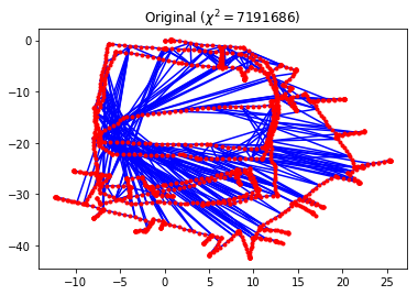
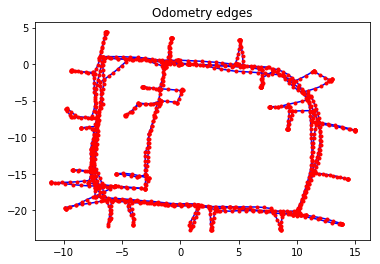
Each edge in this dataset is a constraint that compares the measured \(SE(2)\) transformation between two poses to the expected \(SE(2)\) transformation between them, as computed using the current pose estimates. These edges can be classified into two categories:
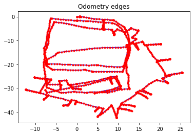
Odometry edges constrain two consecutive vertices, and the measurement for the \(SE(2)\) transformation comes directly from odometry data.
Scan-matching edges constrain two non-consecutive vertices. These scan matches can be computed using, for example, 2-D LiDAR data or landmarks; the details of how these constraints are determined is beyond the scope of this example. This is often referred to as loop closure in the Graph SLAM literature.
We can easily parse out the two different types of edges present in this dataset and plot them.
def parse_edges(g):
    """Split the graph `g` into two graphs, one with only odometry edges and the other with only scan-matching edges.

    Parameters
    ----------
    g : graphslam.graph.Graph
        The input graph

    Returns
    -------
    g_odom : graphslam.graph.Graph
        A graph consisting of the vertices and odometry edges from `g`
    g_scan : graphslam.graph.Graph
        A graph consisting of the vertices and scan-matching edges from `g`

    """
    edges_odom = []
    edges_scan = []

    for e in g._edges:
        if abs(e.vertex_ids[1] - e.vertex_ids[0]) == 1:
            edges_odom.append(e)
        else:
            edges_scan.append(e)

    g_odom = Graph(edges_odom, g._vertices)
    g_scan = Graph(edges_scan, g._vertices)

    return g_odom, g_scan
g_odom, g_scan = parse_edges(g)

print("Number of odometry edges:      {:4d}".format(len(g_odom._edges)))
print("Number of scan-matching edges: {:4d}".format(len(g_scan._edges)))

print("\nχ^2 error from odometry edges:       {:11.3f}".format(g_odom.calc_chi2()))
print("χ^2 error from scan-matching edges:  {:11.3f}".format(g_scan.calc_chi2()))
Number of odometry edges:      1227
Number of scan-matching edges:  256

χ^2 error from odometry edges:             0.232
χ^2 error from scan-matching edges:  7191686.151
g_odom.plot(title="Odometry edges")
g_scan.plot(title="Scan-matching edges")
Optimization
Initially, the pose estimates are consistent with the collected odometry measurements, and the odometry edges contribute almost zero towards the \(\chi^2\) error. However, there are large discrepancies between the scan-matching constraints and the initial pose estimates. This is not surprising, since small errors in odometry readings that are propagated over time can lead to large errors in the robot’s trajectory. What makes Graph SLAM effective is that it allows incorporation of multiple different data sources into a single optimization problem.
g.optimize()
Iteration                chi^2        rel. change
---------                -----        -----------
        0         7191686.3825
        1       320031728.8624          43.500234
        2       125083004.3299          -0.609154
        3          338155.9074          -0.997297
        4             735.1344          -0.997826
        5             215.8405          -0.706393
        6             215.8405          -0.000000
g.plot(title="Optimized")
print("\nχ^2 error from odometry edges:       {:7.3f}".format(g_odom.calc_chi2()))
print("χ^2 error from scan-matching edges:  {:7.3f}".format(g_scan.calc_chi2()))
χ^2 error from odometry edges:       142.189
χ^2 error from scan-matching edges:   73.652
g_odom.plot(title="Odometry edges")
g_scan.plot(title="Scan-matching edges")