Linear–quadratic regulator (LQR) speed and steering control

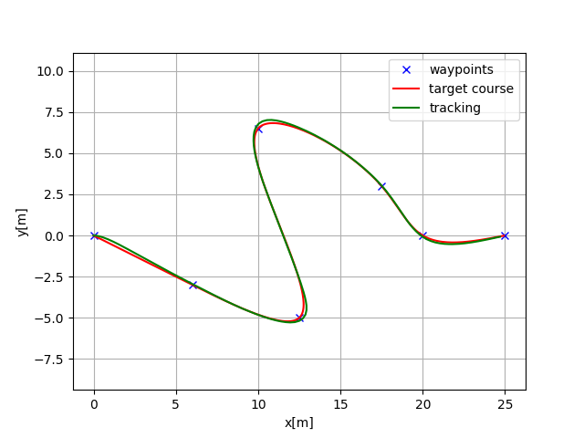
Path tracking simulation with LQR speed and steering control.

https://github.com/AtsushiSakai/PythonRoboticsGifs/raw/master/PathTracking/lqr_speed_steer_control/animation.gif

Overview

The LQR (Linear Quadratic Regulator) speed and steering control model implemented in lqr_speed_steer_control.py provides a simulation for an autonomous vehicle to track:

A desired speed by adjusting acceleration based on feedback from the current state and the desired speed.
A desired trajectory by adjusting steering angle based on feedback from the current state and the desired trajectory.

by only using one LQT controller.

Vehicle motion Model

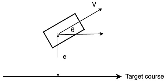
The below figure shows the geometric model of the vehicle used in this simulation:

../../../_images/lqr_steering_control_model.jpg

The e, \({\theta}\), and \(\upsilon\) represent the lateral error, orientation error, and velocity error, respectively, with respect to the desired trajectory and speed. And \(\dot{e}\) and \(\dot{\theta}\) represent the rates of change of these errors.

The \(e_t\) and \(\theta_t\), and \(\upsilon\) are the updated values of e, \(\theta\), \(\upsilon\) and at time t, respectively, and can be calculated using the following kinematic equations:

\[e_t = e_{t-1} + \dot{e}_{t-1} dt\]

\[\theta_t = \theta_{t-1} + \dot{\theta}_{t-1} dt\]

\[\upsilon_t = \upsilon_{t-1} + a_{t-1} dt\]

Where dt is the time difference and \(a_t\) is the acceleration at the time t.

The change rate of the e can be calculated as:

\[\dot{e}_t = V \sin(\theta_{t-1})\]

Where V is the current vehicle speed.

If the \(\theta\) is small,

\[\theta \approx 0\]

the \(\sin(\theta)\) can be approximated as \(\theta\):

\[\sin(\theta) = \theta\]

So, the change rate of the e can be approximated as:

\[\dot{e}_t = V \theta_{t-1}\]

The change rate of the \(\theta\) can be calculated as:

\[\dot{\theta}_t = \frac{V}{L} \tan(\delta)\]

where L is the wheelbase of the vehicle and \(\delta\) is the steering angle.

If the \(\delta\) is small,

\[\delta \approx 0\]

the \(\tan(\delta)\) can be approximated as \(\delta\):

\[\tan(\delta) = \delta\]

So, the change rate of the \(\theta\) can be approximated as:

\[\dot{\theta}_t = \frac{V}{L} \delta\]

The above equations can be used to update the state of the vehicle at each time step.

Control Model

To formulate the state-space representation of the vehicle dynamics as a linear model, the state vector x and control input vector u are defined as follows:

\[x_t = [e_t, \dot{e}_t, \theta_t, \dot{\theta}_t, \upsilon_t]^T\]

\[u_t = [\delta_t, a_t]^T\]

The linear state transition equation can be represented as:

\[x_{t+1} = A x_t + B u_t\]

where:

\(\begin{equation*} A = \begin{bmatrix} 1 & dt & 0 & 0 & 0\\ 0 & 0 & v & 0 & 0\\ 0 & 0 & 1 & dt & 0\\ 0 & 0 & 0 & 0 & 0\\ 0 & 0 & 0 & 0 & 1\\\end{bmatrix} \end{equation*}\)

\(\begin{equation*} B = \begin{bmatrix} 0 & 0\\ 0 & 0\\ 0 & 0\\ \frac{v}{L} & 0\\ 0 & dt \\ \end{bmatrix} \end{equation*}\)