GPS/IMU Fusion Localization with Bias Estimation

This example uses an extended Kalman filter (EKF) to combine body-frame accelerometer and gyroscope measurements with GPS positions in a local metric frame. IMU prediction runs at 20 Hz and GPS correction at 1 Hz. The simulation compares fusion with and without bias estimation and IMU-only dead reckoning along a figure-eight trajectory, including a GPS outage from 20 to 30 seconds.

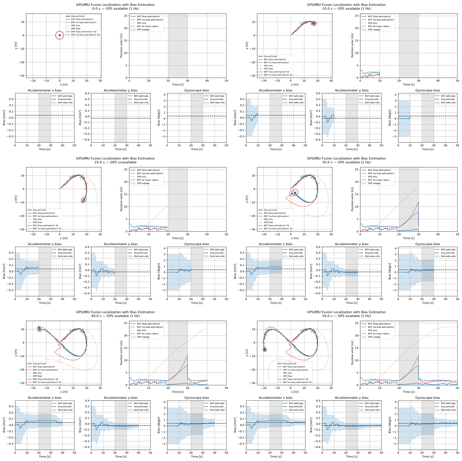
The lower three panels show the EKF’s estimated accelerometer x/y biases (m/s²) and gyroscope bias (deg/s) in blue, with ground truth as black dashed lines. The true biases are 0.04 m/s², -0.03 m/s² and 0.4 deg/s, respectively. Gray shading marks the GPS outage in the error and bias plots.

Covariance-based uncertainty

The path plot shows a 3σ position ellipse centered on each EKF estimate, with markers for the current estimates and ground truth. If \(\lambda_i\) are the eigenvalues of the position covariance \(P_{xy}\), the semi-axis lengths are \(3\sqrt{\lambda_i}\) and the eigenvectors give their directions. This includes the x/y cross-covariance. The ellipse boundary satisfies \((\mathbf{p}-\hat{\mathbf{p}})^T P_{xy}^{-1} (\mathbf{p}-\hat{\mathbf{p}})=9\).

The dashed blue line in the position-error plot tracks the bias-estimating EKF’s ellipse semi-major axis, \(3\sqrt{\lambda_{\max}(P_{xy})}\). It is the ellipse’s enclosing radius, not the standard deviation of the Euclidean position error. An error below this line alone does not guarantee that the true position lies inside the ellipse; direction also matters.

Each bias panel shades \(\hat b_i \pm 3\sqrt{P_{ii}}\), using the matching diagonal element of the estimated state covariance. Gyroscope estimates and standard deviations are both converted from rad/s to deg/s. The estimate is at the center of its band; the true value provides an independent comparison. The plots use the filter covariance directly, so they show uncertainty contracting with GPS corrections and growing during the outage.

For the default seed-0 simulation, ground truth stays within the bias-estimating EKF’s position ellipse and all three bias bands at every sample. The EKF without bias estimation has position errors outside its ellipse during parts of the run. These are results for this synthetic run, not a guarantee of coverage for other data. A 3σ ellipse encloses about 98.9% of an ideal 2D Gaussian, whereas a scalar ±3σ interval encloses about 99.7%; see Matplotlib’s confidence-ellipse explanation.

Assumptions

Motion is restricted to a horizontal plane. The IMU is aligned with the body frame and its acceleration has already been compensated for gravity. GPS positions are expressed in metres, not latitude and longitude. Sensors are time-aligned and co-located. Initial heading and velocity are approximately known. Roll, pitch, altitude, magnetometers and barometers are not modeled.

The example estimates constant or slowly varying accelerometer and gyroscope biases. GPS observes position only, so heading and bias estimation depend on motion and the initial uncertainty; they cannot all be recovered from a stationary position measurement. No real sensor data, outlier rejection or hardware-specific calibration is included.

State and inertial prediction

The eight-dimensional state contains world position, world velocity, heading, two body-frame accelerometer biases and one yaw-rate bias:

\[\mathbf{x} = [p_x, p_y, v_x, v_y, \psi, b_{ax}, b_{ay}, b_\omega]^T.\]

Let \(\mathbf{a}_m\) and \(\omega_m\) be the measured acceleration and yaw rate. With the body-to-world rotation

\[\begin{split}R(\psi)=\begin{bmatrix}\cos\psi&-\sin\psi\\\sin\psi&\cos\psi\end{bmatrix}, \qquad \mathbf{a}_w=R(\psi)(\mathbf{a}_m-\mathbf{b}_a),\end{split}\]

the discrete prediction holds world acceleration constant over one sample:

\[\begin{split}\mathbf{p}^{-} &= \mathbf{p}+\mathbf{v}\Delta t+\tfrac12\mathbf{a}_w\Delta t^2,\\ \mathbf{v}^{-} &= \mathbf{v}+\mathbf{a}_w\Delta t,\\ \psi^{-} &= \operatorname{wrap}(\psi+(\omega_m-b_\omega)\Delta t),\\ \mathbf{b}^{-} &= \mathbf{b}.\end{split}\]

Heading is wrapped to \([-\pi,\pi)\). Define \(\mathbf{j}=[-a_{wy},a_{wx}]^T\). In block order \((\mathbf{p},\mathbf{v},\psi,\mathbf{b}_a,b_\omega)\), the Jacobians are

\[\begin{split}F=\begin{bmatrix} I&\Delta t I&\tfrac12\Delta t^2\mathbf{j}&-\tfrac12\Delta t^2R&0\\ 0&I&\Delta t\mathbf{j}&-\Delta t R&0\\ 0&0&1&0&-\Delta t\\ 0&0&0&I&0\\ 0&0&0&0&1 \end{bmatrix},\qquad G=\begin{bmatrix} \tfrac12\Delta t^2R&0\\ \Delta t R&0\\ 0&\Delta t\\ 0&0\\ 0&0 \end{bmatrix}.\end{split}\]

Covariance propagates as

\[P^{-}=FPF^T+GQ_{\mathrm{imu}}G^T+Q_b.\]

\(Q_{\mathrm{imu}}\) is the covariance of a discrete IMU sample. For bias random-walk standard deviations specified per square root second, the bias block of \(Q_b\) is \(\operatorname{diag}(\sigma_{bax}^2,\sigma_{bay}^2,\sigma_{b\omega}^2)\Delta t\); its other entries are zero. The simulation adds independent Gaussian sensor noise and fixed biases, while the filter allows those biases to vary slowly.

GPS correction and outages

GPS supplies \(\mathbf{z}=[p_x,p_y]^T\) with measurement matrix \(H=[I_2\;0_{2\times6}]\) and covariance \(R_{\mathrm{gps}}=\sigma_{\mathrm{gps}}^2 I_2\).

\[\begin{split}S &= HP^{-}H^T+R_{\mathrm{gps}},\\ K &= P^{-}H^T S^{-1},\\ \mathbf{x}^{+} &= \mathbf{x}^{-}+K(\mathbf{z}-H\mathbf{x}^{-}),\\ P^{+} &= (I-KH)P^{-}(I-KH)^T+KR_{\mathrm{gps}}K^T.\end{split}\]

The gain is computed with a linear solve, and the Joseph covariance update helps preserve numerical symmetry and positive semidefiniteness. Between GPS fixes, and throughout the outage, only IMU prediction is performed. Uncertainty can grow during the outage and decreases when GPS corrections resume.

Comparison without bias estimation

The baseline EKF estimates only \([p_x,p_y,v_x,v_y,\psi]^T\). It assumes zero accelerometer and gyroscope bias, so it uses the raw IMU measurements without bias compensation. Its prediction uses the first five rows and columns of \(F\) and the first five rows of \(G\), with no bias random-walk term. GPS still corrects position, velocity and heading through their cross-covariances. Thus it differs from IMU-only dead reckoning, which never receives GPS corrections.

All three methods use exactly the same IMU samples, including the same nonzero sensor biases and noise. Both EKFs receive the same GPS fixes and outage schedule, and start with the same pose, velocity and corresponding covariance. Only the eight-state EKF estimates and compensates for the biases. The red dashed curves show the five-state EKF without bias estimation.

The analytic reference trajectory is independent of the filter’s discrete integrator. A fixed random seed makes the example reproducible, and the error plot shows each method’s Euclidean position error. These synthetic results are not a real-sensor accuracy claim.

Code

Localization.gps_imu_fusion.gps_imu_fusion.predict(state, covariance, imu, dt=0.05)

Predict at the IMU rate, including sensor noise and bias random walk.

IMU_STD describes independent noise on each discrete IMU sample, while BIAS_RW_STD describes continuous bias random walk per sqrt(second). A five-state filter assumes zero bias and has no bias random walk.

Localization.gps_imu_fusion.gps_imu_fusion.update_gps(state, covariance, position)

Correct the predicted state when a new 2D GPS position is available.

GPS observes only position. Velocity, heading and biases are corrected through cross-covariances accumulated during IMU prediction.

Localization.gps_imu_fusion.gps_imu_fusion.simulate(duration=50.0, seed=0, gps_outage=(20.0, 30.0))

Run a deterministic simulation with multi-rate sensors.

GPS outages cover [start, end); pass None for uninterrupted GPS. Truth is computed analytically, independently of the filter’s discrete integrator. All three estimates share the same biased, noisy measurements and start with the known initial pose/velocity. The eight-state EKF starts with zero estimated bias; the five-state EKF and dead reckoning assume zero bias.

References

• Oliver J. Woodman, An introduction to inertial navigation, University of Cambridge, 2007

• Extended Kalman Filter Localization