Cubic spline planning

Spline curve continuity

Spline curve smoothness is depending on the which kind of spline model is used.

The smoothness of the spline curve is expressed as \(C_0, C_1\), and so on.

This representation represents continuity of the curve. For example, for a spline curve in two-dimensional space:

• \(C_0\) is position continuous

• \(C_1\) is tangent vector continuous

• \(C_2\) is curvature vector continuous

as shown in the following figure:

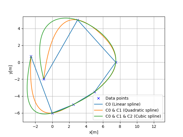
Cubic spline can generate a curve with \(C_0, C_1, C_2\).

1D cubic spline

Cubic spline interpolation is a method of smoothly interpolating between multiple data points when given multiple data points, as shown in the figure below.

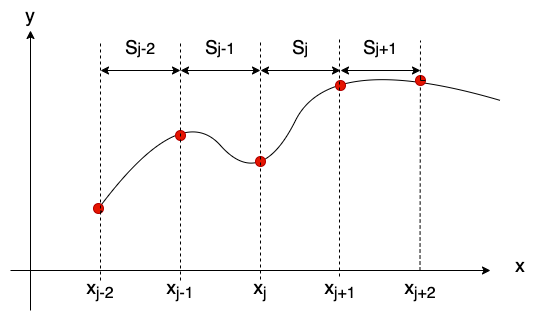
It separates between each interval between data points.

The each interval part is approximated by each cubic polynomial.

The cubic spline uses the cubic polynomial equation for interpolation:

\(S_j(x)=a_j+b_j(x-x_j)+c_j(x-x_j)^2+d_j(x-x_j)^3\)

where \(x_j < x < x_{j+1}\), \(x_j\) is the j-th node of the spline, \(a_j\), \(b_j\), \(c_j\), \(d_j\) are the coefficients of the spline.

As the above equation, there are 4 unknown parameters \((a,b,c,d)\) for one interval, so if the number of data points is \(N\), the interpolation has \(4N\) unknown parameters.

The following five conditions are used to determine the \(4N\) unknown parameters:

Constraint 1: Terminal constraints

\(S_j(x_j)=y_j\)

This constraint is the terminal constraint of each interval.

The polynomial of each interval will pass through the x,y coordinates of the data points.

Constraint 2: Point continuous constraints

\(S_j(x_{j+1})=S_{j+1}(x_{j+1})=y_{j+1}\)

This constraint is a continuity condition for the boundary of each interval.

This constraint ensures that the boundary of each interval is continuous.

Constraint 3: Tangent vector continuous constraints

\(S'_j(x_{j+1})=S'_{j+1}(x_{j+1})\)

This constraint is a continuity condition for the first derivative of the boundary of each interval.

This constraint makes the vectors of the boundaries of each interval continuous.

Constraint 4: Curvature continuous constraints

\(S''_j(x_{j+1})=S''_{j+1}(x_{j+1})\)

This constraint is the continuity condition for the second derivative of the boundary of each interval.

This constraint makes the curvature of the boundaries of each interval continuous.

Constraint 5: Terminal curvature constraints

\(S''_0(0)=S''_{n+1}(x_{n})=0\).

The constraint is a boundary condition for the second derivative of the starting and ending points.

Our sample code assumes these terminal curvatures are 0, which is well known as Natural Cubic Spline.

How to calculate the unknown parameters \(a_j, b_j, c_j, d_j\)

Step1: calculate \(a_j\)

Spline coefficients \(a_j\) can be calculated by y positions of the data points:

\(a_j = y_i\).

Step2: calculate \(c_j\)

Spline coefficients \(c_j\) can be calculated by solving the linear equation:

\(Ac_j = B\).

The matrix \(A\) and \(B\) are defined as follows:

\[\begin{split}A=\left[\begin{array}{cccccc} 1 & 0 & 0 & 0 & \cdots & 0 \\ h_{0} & 2\left(h_{0}+h_{1}\right) & h_{1} & 0 & \cdots & 0 \\ 0 & h_{1} & 2\left(h_{1}+h_{2}\right) & h_{2} & \cdots & 0 \\ 0 & 0 & h_{2} & 2\left(h_{2}+h_{3}\right) & \cdots & 0 \\ 0 & 0 & 0 & h_{3} & \ddots & \\ \vdots & \vdots & & & & \\ 0 & 0 & 0 & \cdots & 0 & 1 \end{array}\right]\end{split}\]

\[\begin{split}B=\left[\begin{array}{c} 0 \\ \frac{3}{h_{1}}\left(a_{2}-a_{1}\right)-\frac{3}{h_{0}}\left(a_{1}-a_{0}\right) \\ \vdots \\ \frac{3}{h_{n-1}}\left(a_{n}-a_{n-1}\right)-\frac{3}{h_{n-2}}\left(a_{n-1}-a_{n-2}\right) \\ 0 \end{array}\right]\end{split}\]

where \(h_{i}\) is the x position distance between the i-th and (i+1)-th data points.

Step3: calculate \(d_j\)

Spline coefficients \(d_j\) can be calculated by the following equation:

\(d_{j}=\frac{c_{j+1}-c_{j}}{3 h_{j}}\)

Step4: calculate \(b_j\)

Spline coefficients \(b_j\) can be calculated by the following equation:

\(b_{i}=\frac{1}{h_i}(a_{i+1}-a_{i})-\frac{h_i}{3}(2c_{i}+c_{i+1})\)

How to calculate the first and second derivatives of the spline curve

After we can get the coefficients of the spline curve, we can calculate

the first derivative by:

\(y^{\prime}(x)=b+2cx+3dx^2\)

the second derivative by:

\(y^{\prime \prime}(x)=2c+6dx\)

These equations can be calculated by differentiating the cubic polynomial.

Code Link

This is the 1D cubic spline class API:

class PathPlanning.CubicSpline.cubic_spline_planner.CubicSpline1D(x, y)

1D Cubic Spline class

Parameters:

• x (list) – x coordinates for data points. This x coordinates must be sorted in ascending order.

• y (list) – y coordinates for data points

Examples

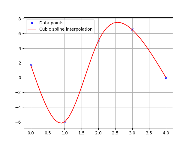
You can interpolate 1D data points.

>>> import numpy as np
>>> import matplotlib.pyplot as plt
>>> x = np.arange(5)
>>> y = [1.7, -6, 5, 6.5, 0.0]
>>> sp = CubicSpline1D(x, y)
>>> xi = np.linspace(0.0, 5.0)
>>> yi = [sp.calc_position(x) for x in xi]
>>> plt.plot(x, y, "xb", label="Data points")
>>> plt.plot(xi, yi , "r", label="Cubic spline interpolation")
>>> plt.grid(True)
>>> plt.legend()
>>> plt.show()

calc_first_derivative(x)

Calc first derivative at given x.

if x is outside the input x, return None

Parameters:

x (float) – x position to calculate first derivative.

Returns:

dy – first derivative for given x.

Return type:

float

calc_position(x)

Calc y position for given x.

if x is outside the data point’s x range, return None.

Parameters:

x (float) – x position to calculate y.

Returns:

y – y position for given x.

Return type:

float

calc_second_derivative(x)

Calc second derivative at given x.

if x is outside the input x, return None

Parameters:

x (float) – x position to calculate second derivative.

Returns:

ddy – second derivative for given x.

Return type:

float

calc_third_derivative(x)

Calc third derivative at given x.

if x is outside the input x, return None

Parameters:

x (float) – x position to calculate third derivative.

Returns:

dddy – third derivative for given x.

Return type:

float

2D cubic spline

Data x positions needs to be mono-increasing for 1D cubic spline.

So, it cannot be used for 2D path planning.

2D cubic spline uses two 1D cubic splines based on path distance from the start point for each dimension x and y.

This can generate a curvature continuous path based on x-y waypoints.

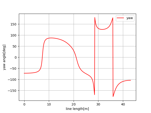
Heading angle of each point can be calculated analytically by:

\(\theta=\tan ^{-1} \frac{y’}{x’}\)

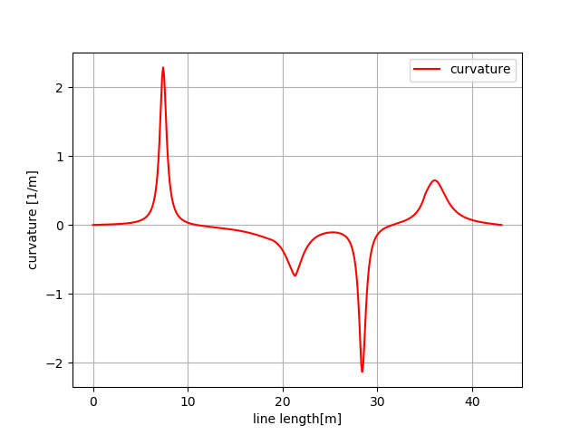
Curvature of each point can be also calculated analytically by:

\(\kappa=\frac{y^{\prime \prime} x^{\prime}-x^{\prime \prime} y^{\prime}}{\left(x^{\prime2}+y^{\prime2}\right)^{\frac{2}{3}}}\)

Code Link

class PathPlanning.CubicSpline.cubic_spline_planner.CubicSpline2D(x, y)

Cubic CubicSpline2D class

Parameters:

• x (list) – x coordinates for data points.

• y (list) – y coordinates for data points.

Examples

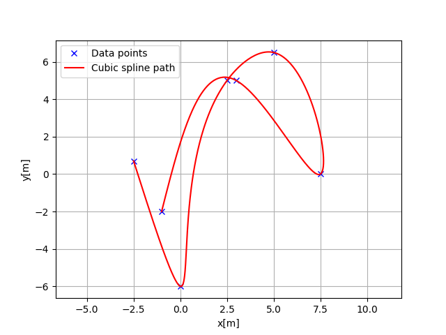
You can interpolate a 2D data points.

>>> import matplotlib.pyplot as plt
>>> x = [-2.5, 0.0, 2.5, 5.0, 7.5, 3.0, -1.0]
>>> y = [0.7, -6, 5, 6.5, 0.0, 5.0, -2.0]
>>> ds = 0.1  # [m] distance of each interpolated points
>>> sp = CubicSpline2D(x, y)
>>> s = np.arange(0, sp.s[-1], ds)
>>> rx, ry, ryaw, rk = [], [], [], []
>>> for i_s in s:
...     ix, iy = sp.calc_position(i_s)
...     rx.append(ix)
...     ry.append(iy)
...     ryaw.append(sp.calc_yaw(i_s))
...     rk.append(sp.calc_curvature(i_s))
>>> plt.subplots(1)
>>> plt.plot(x, y, "xb", label="Data points")
>>> plt.plot(rx, ry, "-r", label="Cubic spline path")
>>> plt.grid(True)
>>> plt.axis("equal")
>>> plt.xlabel("x[m]")
>>> plt.ylabel("y[m]")
>>> plt.legend()
>>> plt.show()

>>> plt.subplots(1)
>>> plt.plot(s, [np.rad2deg(iyaw) for iyaw in ryaw], "-r", label="yaw")
>>> plt.grid(True)
>>> plt.legend()
>>> plt.xlabel("line length[m]")
>>> plt.ylabel("yaw angle[deg]")

>>> plt.subplots(1)
>>> plt.plot(s, rk, "-r", label="curvature")
>>> plt.grid(True)
>>> plt.legend()
>>> plt.xlabel("line length[m]")
>>> plt.ylabel("curvature [1/m]")

calc_curvature(s)

calc curvature

Parameters:

s (float) – distance from the start point. if s is outside the data point’s range, return None.

Returns:

k – curvature for given s.

Return type:

float

calc_curvature_rate(s)

calc curvature rate

Parameters:

s (float) – distance from the start point. if s is outside the data point’s range, return None.

Returns:

k – curvature rate for given s.

Return type:

float

calc_position(s)

calc position

Parameters:

s (float) – distance from the start point. if s is outside the data point’s range, return None.

Returns:

• x (float) – x position for given s.

• y (float) – y position for given s.

calc_yaw(s)

calc yaw

Parameters:

s (float) – distance from the start point. if s is outside the data point’s range, return None.

Returns:

yaw – yaw angle (tangent vector) for given s.

Return type:

float

References

• Cubic Splines James Keesling

• Curves and Splines